Should you go for it? A base steal predictor for the MLB

One of the most exciting things in baseball is the base steal. There are two outcomes, if the base runner times it properly:

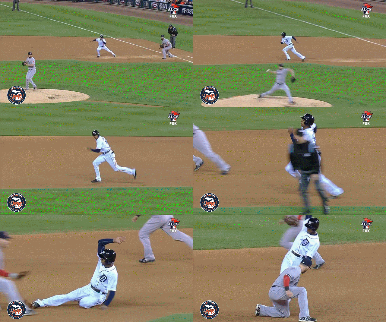
or they don’t:

Sometimes even something amazing can happen, look at this play by Jayson Werth:

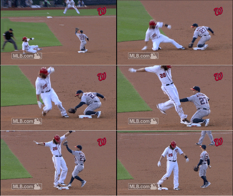
Base stealing is a calculated gamble, where game situation dictates the chances for success. To make the decision on whether or not go for it requires sound judgement from both the base runner and the manager, judgement only gained from playing decades of high level baseball. However, what if this decision could be made just with the click of a button? I decided to try to do this by building a predictive model for my 3rd Metis project and created a Flask app that was deployed on Heroku.

Data:

Acquiring Data:

To build this model I needed many examples of base stealing situations and their outcomes. Luckily Kaggle had such a data set that was provided by Sportsradar. Hosted on Google’s Bigquery platform, this MLB data set contained information on every play from the 2016 season. I ended up uploading this data to a PostgreSQL server as the initial dataset contained 760,000+ rows and 145 features, which would be too large to load into my local memory.

One initial quirk in exploring this data set was trying to pull just base steal events. Initially I tried to find them by just doing a wildcard search for ‘steal’ in the descriptions:

  SELECT *  
  FROM baseball  
  WHERE description LIKE '%steal%';

However this query was too small as it only returned 500 entries. As an example, the top 10 teams leading the 2017 MLB season in stolen bases had totals of:

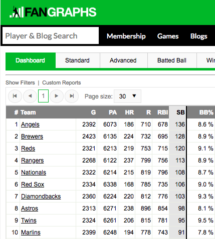
So only 500 entires would be too low. Digging deeper, I discovered that multiple base stealing events were missing information in their descriptions. Thus, I ended up querying the steal events by using:

    SELECT *
    FROM baseball
    WHERE rob1_outcomeid LIKE '%CS%'
    OR rob1_outcomeid LIKE '%SB%'
    OR rob2_outcomeid LIKE '%CS%'
    OR rob2_outcomeid LIKE '%SB%'
    OR rob3_outcomeid LIKE '%CS%'
    OR rob3_outcomeid LIKE '%SB%';

As each rob (runner on base) had an outcome id, by looking for the presence of either ‘SB’ (stolen base) or ‘CS’ (caught stealing) I was able to grab the steal events.

With 145 features, there was a lot of information available for each play. While a lot of these features would end up not being predictive, there were a couple features that I thought were informative but not reflective of a real-time situation. For example, information on the pitch type, pitch speed, and pitch location would be very useful for a base runner. These features would allow a base runner to estimate approximately how much time they had to reach the next base. However, in the real world this information would not be available to the runner or manager so I decided to restrict these features from the model.

As a substitute, I joined my dataset with player statistics from Fangraphs. Specifically I utilized the pitcher pitch type distribution statistics as a proxy for the pitch type and velocity, while the hitter plate discipline statistics was a proxy for pitch location. This is a reflective of how a base runner would be guessing what pitch the pitcher would throw based on their past tendencies.

Data Cleaning:

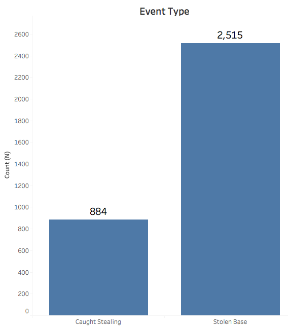
While the Sportsradar data was comprehensive, I still needed to clean the data. The dataset contained 760,000+ entries which I had to filter to only base steals events. I took out any pickoff events or events in the post season. My reasoning was that pickoffs are different from a normal steal attempt and that post season behavior is different from regular season behavior. These data cuts left me with 3000+ base steal events:

Many features like gameID, attendance, venueName were also excluded as I felt they would not be predictive.

Data Imputation:

Besides subsetting there were entries where the pitcher or hitter stats were missing. This occurred when the listed pitcher or hitter were missing from the Fangraphs stats. This was to be expected because of the year difference (2016 vs 2015) in data sets. It is reasonable to assume that there are 2016 players that did not play in 2015 (like rookies). To account for these missing values, I ended up imputing those features with the respective median value as calculated from the training data.

Feature Generation:

With the large number of categorical variables, I ended up having to dummify a lot of features to make them interpretable to my models. In doing so, I made sure to not fall for the dummy variable trap (DVT). For instance, to determine the handedness of a hitter I created one column ‘is_hitter_R’ instead of two as that would fall into the DVT for this data set (there was only one hitter that was ambidextrous).

The other type of feature engineering that I utilized involved box-cox transformations. Many of the player statistic features were not normally distributed and tightly grouped, so to rectify that I applied a box-cox transformation where each feature was transformed with an optimized lambda.

Modeling:

Optimization Metric:

As a manager, there would be multiple possible metrics this application could try to optimize for. First would be to maximize the number base steals (minimizing false negatives), however such a strategy could be too risky as that could result in too many outs. Second would be to minimize caught stealing events (minimizing false positives), however this strategy could be too passive and not take advantage of possible scoring opportunities. Instead I decided to optimize for F1 which would bring a balanced approach:

Model Selection:

In maximizing F1 after experimenting with other models, two models performed the best: Logistic Regression (LR) and Gradient Boosted Trees:

Both models ended up with similar F1 scores on the training set. Therefore I chose a LR model for two reasons: LR model’s feature importance is easier to interpret and the run time of the LR model was faster. The latter would be important if I was trying to deploy a real time app.

Feature Importance:

From the LR model, these were the most important features for each outcome:

BC refers to the box-cox representation of the feature

The most dominant feature was whether or not the base runner was on 1st base. Out of all of the features it appeared to be twice as predictive as the next closest. This makes sense physically as a base runner on first base would have a better chance to steal a base one on any other base.

Model Performance:

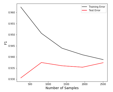
My LR model’s test F1 score was 0.924. The small difference from the test score meant that my model was generalizing well to new data and not overfitting. This was reinforced by the learning curve:

Retraining the model on the full data set, it was able to generate the following confusion matrix:

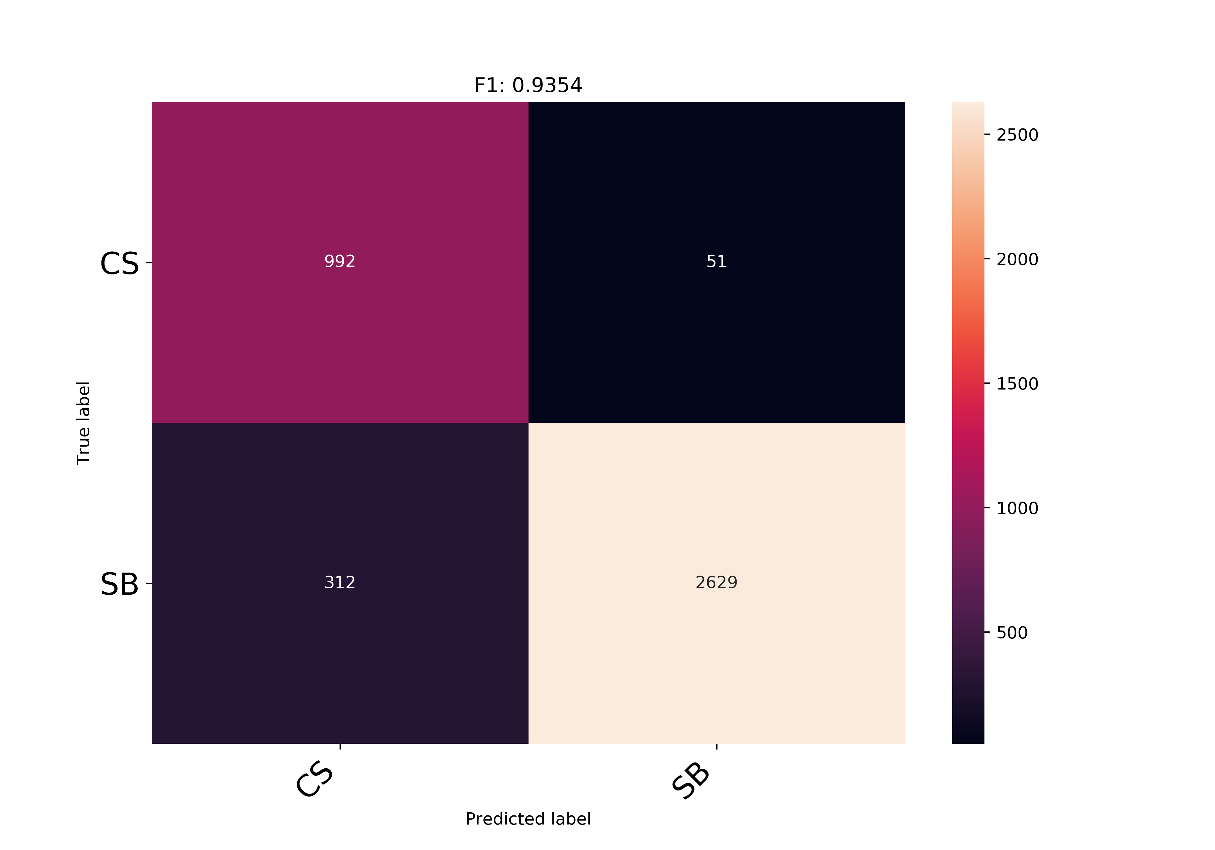
With a final F1 score of 0.9354, the model performance ended up right between the training and test F1 scores. One way to interpret these results would be to equate the number of caught stealing (CS) events to runs that would have been saved. With 922 CS events that the model was able to classify, a ballpark estimate of runs saved would be 123 runs. I utilized the this runs table I found online to translate the game situation of each steal attempt (dividing by 2 to be conservative).

With this model I also ended up building an interactive Flask app that would do predictions based on user selected inputs as shown:

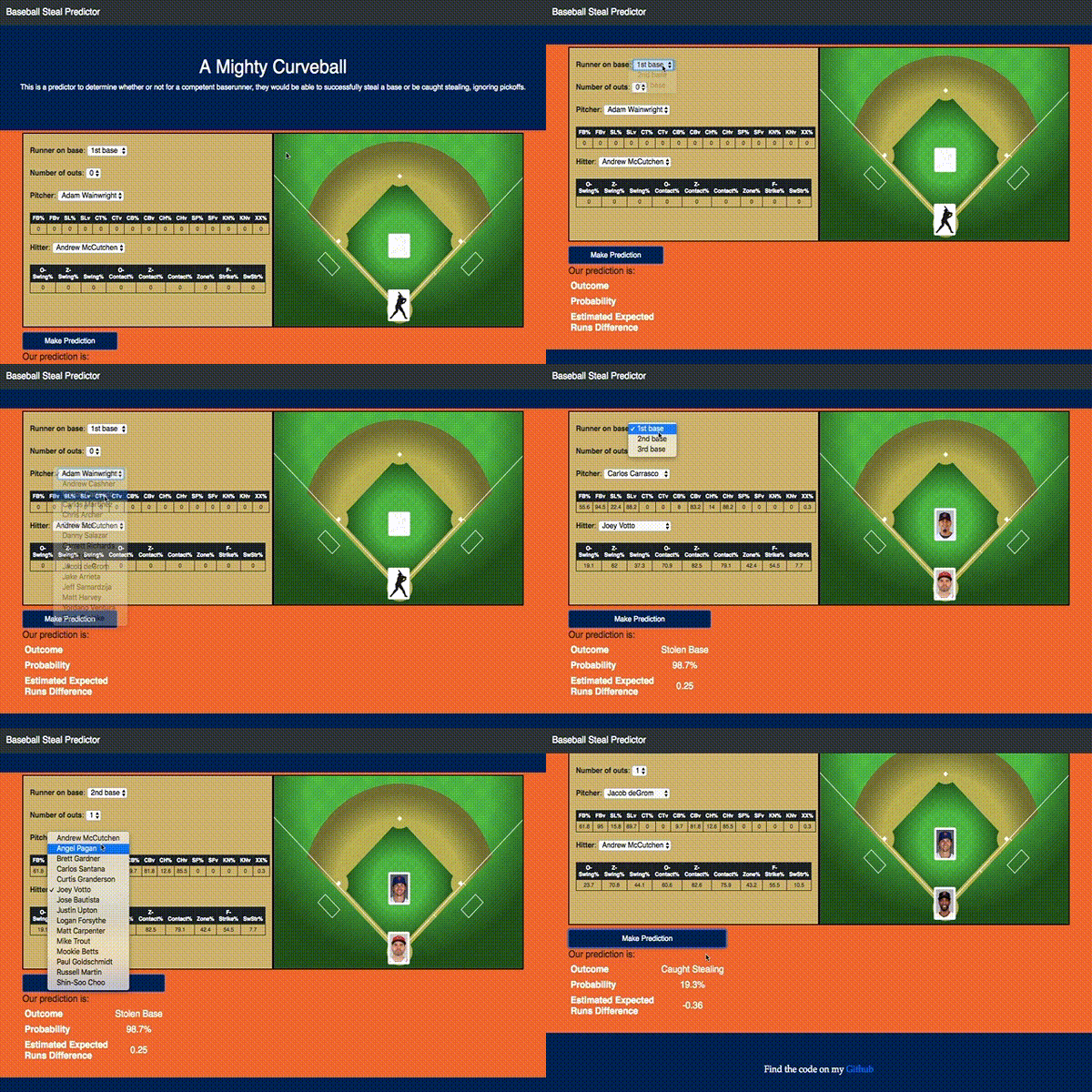
If you would like to play with it yourself you can access it here.

Future Work:

While I ended up with a working model, there were a few improvements that I could implement if I wanted to extend this project further:

• Multiple base runners: With the current model, it is only accurate for predicting singular baserunner events. While it can predict the successfulness of a base being stolen if there are multiple baserunners, the predictions don’t account for multiple outs.

• Runner information: My model currently does not account for the base runner’s ability. Thus, I would have like to include base running statistics for the runner on base. Some statistics that could be utilized would be the amount of bases that a baserunner had stolen the previous year and metrics like their 40 yard dash time.

• More data: I believe access to more data would help improve this model greatly. If I had gotten data from other MLB seasons to rectify the imbalance between CS and SB events, I believe that I would have found more predictive features.

The code and data for this model and Flask app are available at my Github repo.

Is That New Lunch Spot Overpriced?

How many times have you gone to a new restaurant where every dish seems overpriced? Consider when your regular lunch spot is offering a new special, is it even worth trying? Are restaurants trying to upcharge you on things like decor or reputation? What if you had a model that could you help predict the likelihood of that?

I decided to design this model for my 2nd Metis project, where I would utilize linear regression to predict the price of a lunch dish based on the information that one could gather from the restaurant menu.

Data

To train this model, there were three types of data that were obtained:

Restaurant Data

To put constraints on types of restaurants for the dataset, only restaurants in San Francisco, CA were picked. Also these restaurants would focus on 6 types of cuisines that were a diverse representative of lunch choices in SF:

1. American
2. Mexican
3. Mediterranean
4. African
5. Pakistani
6. Creole & Cajun

As there was no freely available database of restaurant menu data, I had to resort other tactics. Using BeautifulSoup (BS4) I was able to obtain the menu information for over 1000 restaurants in SF from a restaurant menu aggregator. These 1000 restaurants in turn gave me over 16,000 data points for dishes at different price points.

Ingredient Data

In order establish meaning from the restaurant menu text, my model would need a reference list of important words. Thus using BS4, I obtained a base ingredient list from some recipe related websites that contained 600+ unique food-related nouns.

Demographic Data

I was curious to see if there was any correlation between dish price and the neighborhood that each restaurant resided in. Luckily there were addresses and geolocation information for each restaurant in the dataset. As a proxy for neighborhood I used a restaurant’s zipcode instead, as there was demographic data for each zipcode in SF from the US Census. I specifically used the 2016 American Community Survey (ACS) and the 2016 Economic Census.

Exploratory Data Analysis (EDA)

With the data in hand there were three aspects that I focused on during the EDA process:

Data Cleaning

In examining the raw data there was some necessary cleaning:

1. Missing Info: For certain entries, the dish price was not listed. This was generally the case when dishes were all grouped and set at the same price (i.e. dim sum). For these dishes I ended up dropping them from the dataset.

2. Outliers: Some dishes were much more expensive than expected based off their ingredients and stuck out as outliers. Digging in deeper, I discovered that many of these dishes were actually labeled as sharing platters or group meals. Because I was focusing on a meal for one, I ended up dropping these entries from the dataset.

Data Cut

As I wanted to restrict my model to predict the prices of dishes at lunch, I ended up removing any dishes that cost more than $20 or less than $7. However, even with this subset there were still 10,000+ data points.

Feature Generation

With the restaurant text gathered, there was flexibility in feature generation using NLP (Natural Language Processing) such as:

1. By identifying nouns in the dish text and cross-referencing with the base ingredient list, the model was able to identify food-related nouns. These nouns were then fed into NLTK’s WordNet corpus reader to identify base words (needed to account for tenses). These nouns were our “ingredients” and each was assigned as a categorical variable.

2. The frequency that each ingredient appeared in high-cost and low-cost dishes from the training set was used to generate a list of high-cost and low-cost ingredients. The frequency that these price-categorized ingredients appeared in each dish were also used as features in the model.

Model Selection

As price was what my model’s target variable, the parameter I decided to optimize for was RMSE (root mean square error). RMSE was the appropriate metric because the RMSE value would be translated as the standard error for any predicted price. As an example, if my model had a test RMSE of $2.00 and the predicted price was $4.00 that would mean my price prediction would be $4.00 ± $2.00

In trying to improve my RMSE there were a couple of modifications that I did to my base linear regression model:

Data Transformations

As seen previously, the pricing data was very skewed. By applying a Box-Cox transformation I was able to transform the data to be more Gaussian in nature.

Regularization

With about 600 starting features in my model, regularization was sorely needed in order to help reduce the number of features. By using Lasso regularization, I was able to subtract 130 features from my model. Most likely, if I was more aggressive in reducing the number of features during the cross-validation process even more features would have been dropped.

Important Features

With regards to the most predictive features, there a mixture of expected and unexpected results. The most predictive features were:

While restaurant types (Mexican and Jerk) and specific ingredients were expectedly predictive, a real surprise was dish text length. Behind expensive ingredients (like crab, lobster, and duck) dish text length was actually the 4th strongest positive predictor where it demonstrated a log-squared relation. That actually made sense because more expensive restaurants would generally be more verbose and embellish dish descriptions.

One more note was that demographic features did not end up being particularly predictive, so any information regarding restaurant location ended up being dropped from the model.

Model Performance

My final model ended up having a train RMSE of $2.44 and a test RMSE of $2.63.

As both values are similar and the residual plots are similar in shape, I believe my model was generalizing well and not overfitting.

So bringing this back to the original question, if you went to the restaurant Best Mexican and ordered a burrito that contained:

• Steak
• Salsa
• Cheese
• Tortilla
• Beans

My model would predict a price of $7.80. If Best Mexican was charging anything more than $10.43 then they would be ripping you off.

Future Improvements

If I had more time and could redo this model, a couple of improvements I think would further minimize the RMSE would be to:

1. Capture more descriptive text features
   • Cooking descriptors (fried vs. baked), multi-word ingredients (i.e. goat cheese), and brand names aren’t currently captured
2. Create temporal features
   • Different groups of dishes take different amounts of time (i.e. burritos vs pies) and this labor cost is currently not captured in the price prediction.
3. Select a better model
   • If I were to choose a different model I would utilize a Random Forest regressor due to the high number of categorical features in my model
   • Test RMSE using Random Forest is $2.41

The code and data for this model are available at my Github repo.